Reproducible evidence
Checking the calculations.
These cases are generated by the same propagation and event-location functions used by the planner. The table is a compact view of behavior that is also covered by the project’s automated checks.
Reference case
Earth constants and thresholds.
Every case below uses the Earth constants in the body catalog and fixed initial states committed with the report generator. Distances are kilometres, velocities are kilometres per second, and time is seconds.
- Earth radius
- 6378.137 km
- Earth μ
- 398600.4418 km³/s²
- Report generator
- buildValidationReport()
- Cases
- 5 representative checks
The analytical circular period and vis-viva maneuver calculations are independent references for the numerical propagation. They are not a second numerical implementation.
Cases generated from code
Representative checks.
Circular orbit returns after one period
passPropagate a 7,000 km circular state for the analytical Kepler period.
- Analytical period
- 5828.517 s
- Position error (limit 1e-5 km)
- 1.373e-11 km
- Velocity error (limit 1e-8 km/s)
- 0.000e+0 km/s
- Relative energy drift
- 0.00e+0
- Relative angular-momentum drift
- 0.00e+0
Forward propagation reverses cleanly
passPropagate a 3D state forward 4,321.5 s, then propagate the result backward by the same duration.
- Position error (limit 1e-5 km)
- 9.118e-12 km
- Velocity error (limit 1e-8 km/s)
- 1.071e-14 km/s
- Forward solver
- converged
- Reverse solver
- converged
Analytical prograde burn raises apoapsis
passAdd 0.1 km/s at 400 km altitude and compare vis-viva prediction with propagation at the opposite apsis.
- Burn
- 0.100 km/s prograde
- Predicted apoapsis
- 765.5 km altitude
- Simulated apoapsis
- 765.5 km altitude
- Absolute difference
- 2.728e-12 km (limit 0.1 km)
Near-parabolic, parabolic, and hyperbolic coasts
passPropagate three 20,000 s states around and above escape speed, requiring finite output and energy drift below 1e−9.
- Near-parabolic
- finite / converged
- Parabolic
- finite / converged
- Hyperbolic
- finite / converged
Impact, escape, and solver failure are explicit
passLocate radius events and deliberately exhaust the subdivision budget; do not return a guessed state.
- Impact event
- 643.836 s at Earth radius
- Escape display crossing
- 12954.385 s at 80,000 km
- Failure reason
- non-convergence
- Returned state after failure
- none
Independent checks
A second numerical method.
SciPy 1.17.1 DOP853 integrates Cartesian acceleration independently of the universal-variable solver. Across inclined, eccentric, parabolic and hyperbolic cases, maximum position error must remain below 0.0001 km and velocity error below 0.0000001 km/s.
- two-body-inclined: 1.185e-6 km; 1.411e-9 km/s. Pass.
- two-body-eccentric: 1.580e-7 km; 1.683e-10 km/s. Pass.
- two-body-parabolic: 9.950e-8 km; 1.326e-11 km/s. Pass.
- two-body-hyperbolic: 1.107e-7 km; 1.311e-11 km/s. Pass.
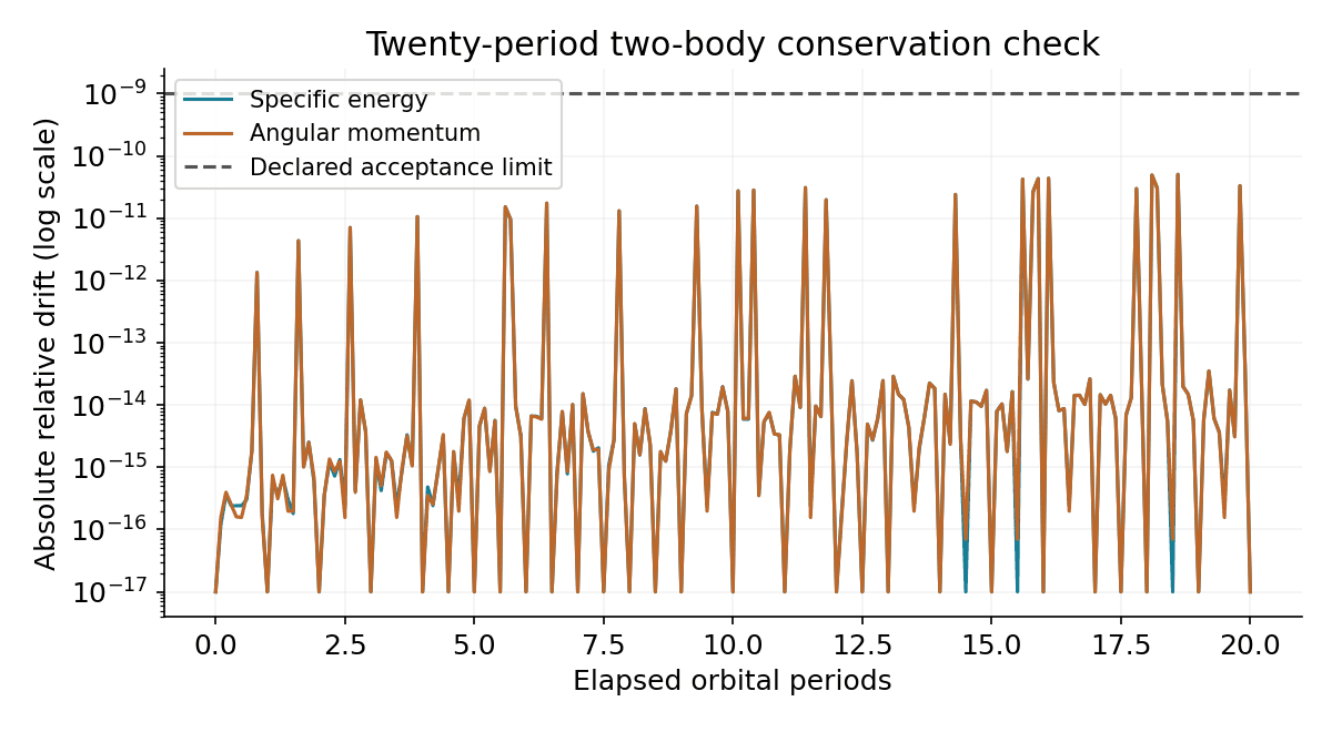
Generating revision: 18ef9f4a958f. Exact source hashes, initial conditions, tolerances, and all samples accompany the report.
Download numerical report · Download reproducibility package
How to read this
Numerical checks answer a narrower question.
Small state and invariant errors show that the implementation behaves consistently for these scenarios. They do not show that a two-body model is physically complete. Numerical error and model error are different questions.
The Earth J2 investigation separates model divergence from numerical error using declared thresholds, independent reference cases, and step convergence.
Read the methods and assumptions →