Investigation · Earth’s equatorial bulge
When does two-body gravity stop being close enough?
Earth’s gravity is slightly different from that of a point mass. This experiment adds only the leading oblateness term, J2, and asks when the two predictions separate by 10 km. The hypothesis is that the lower orbits will cross that threshold sooner than the high orbit over the same 24 hours.
Same start. Two gravity models.
Both spacecraft start at the same position and velocity. The initial speed is circular in the point-mass model. Adding J2 changes the subsequent motion; it does not change the initial state.
- Position separation
- 1112.24 km
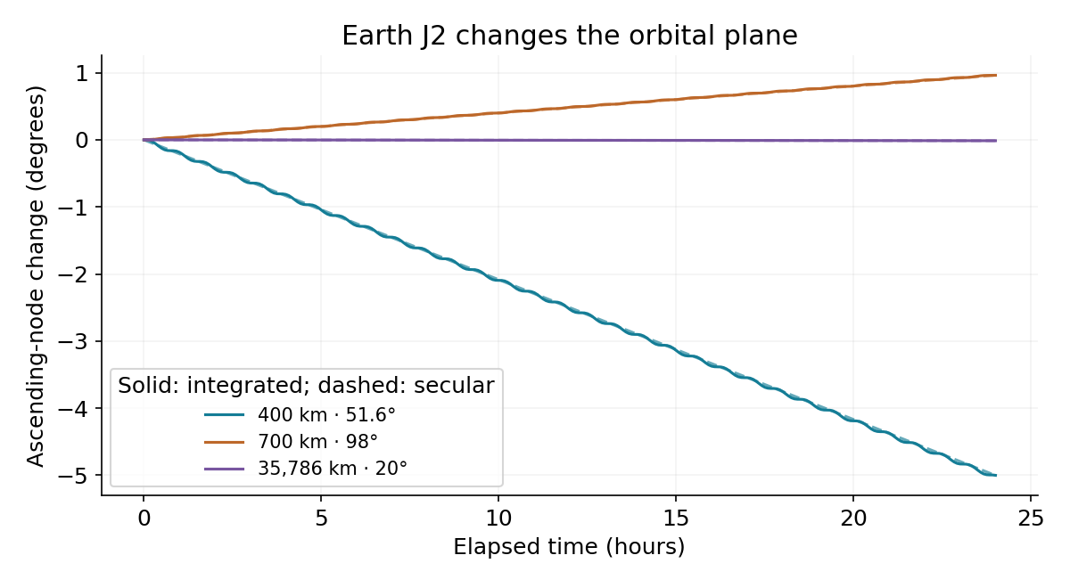
- J2 ascending-node change
- -5.001°
- First sample above 10 km
- 0.42 hours
- J2 energy drift
- 1.59e-11
For this experiment, “close enough” means position separation below 10 km. It is an illustrative threshold chosen before calculation, not a navigation requirement. Samples are five minutes apart, so the first crossing is bracketed between that sample and the preceding one.
Hourly values as a table
| Hours | Separation (km) | Node change (deg) |
|---|---|---|
| 0 | 0.000 | 0.0000 |
| 1 | 54.177 | -0.1850 |
| 2 | 76.668 | -0.4334 |
| 3 | 143.642 | -0.6434 |
| 4 | 188.947 | -0.8131 |
| 5 | 202.886 | -1.0458 |
| 6 | 280.102 | -1.2807 |
| 7 | 330.009 | -1.4510 |
| 8 | 336.348 | -1.6586 |
| 9 | 406.771 | -1.9082 |
| 10 | 469.590 | -2.0947 |
| 11 | 482.081 | -2.2778 |
| 12 | 528.176 | -2.5260 |
| 13 | 599.505 | -2.7378 |
| 14 | 637.789 | -2.9069 |
| 15 | 654.324 | -3.1383 |
| 16 | 715.815 | -3.3743 |
| 17 | 794.315 | -3.5455 |
| 18 | 794.408 | -3.7512 |
| 19 | 822.722 | -4.0008 |
| 20 | 940.077 | -4.1893 |
| 21 | 949.847 | -4.3710 |
| 22 | 932.735 | -4.6178 |
| 23 | 1066.697 | -4.8321 |
| 24 | 1112.236 | -5.0008 |
What the runs show
In these three scenarios, the first samples above 10 km occur at 25 minutes (400 km · 51.6°), 40 minutes (700 km · 98°), 740 minutes (35,786 km · 20°). This supports the hypothesis for the chosen starts and threshold. Separation can oscillate; crossing once does not mean the paths remain more than 10 km apart forever.
The ascending node regresses in the prograde cases and advances in the retrograde case. Position error alone does not identify the effect: the node plot below makes the plane’s slow rotation visible.
Separate model differences from numerical error
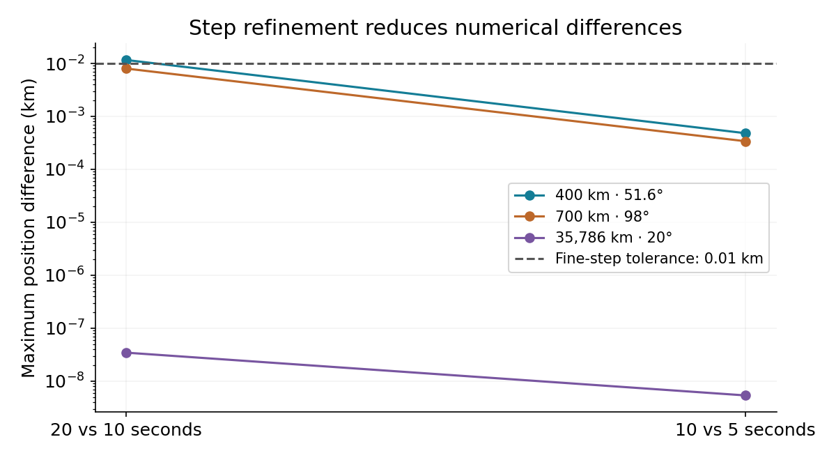
The J2 integration uses classical RK4 at 5-second steps. Repeating at 10 and 20 seconds measures step sensitivity. A separately implemented Cartesian model integrated by SciPy 1.17.1 DOP853 supplies the reference. The tests below use the full set of five-minute samples over 24 hours.
| Scenario | Position vs reference (km) | Velocity vs reference (km/s) | 5 vs 10 s position (km) | Result |
|---|---|---|---|---|
| 400 km · 51.6° | 2.366e-5 | 2.681e-8 | 4.812e-4 | Pass |
| 700 km · 98° | 1.708e-5 | 1.809e-8 | 3.394e-4 | Pass |
| 35,786 km · 20° | 9.109e-9 | 6.261e-13 | 5.387e-9 | Pass |
Declared tolerances: position below 0.01 km, velocity below 10⁻⁵ km/s, 5-to-10-second position difference below 0.01 km, relative drift in J2 energy and axial angular momentum below 10⁻⁸, and fitted node-rate agreement within 0.1°/day of the first-order estimate. Reference step/tolerance sensitivity must remain below 10⁻⁴ km.
The high-orbit integration is close to the floating-point floor. Its convergence ratio should not be interpreted as a clean measurement of RK4 order. The independent comparison and absolute tolerances are the more useful checks there.
Equations, constants, and limits
Both models use μ = 398600.4418 km³/s² and R = 6378.137 km. The comparison uses J2 = 0.00108262668, a fixed teaching value. The inertial +Z axis is aligned with the assumed fixed Earth pole. No calendar epoch, polar motion, atmosphere, higher gravity harmonics, third bodies, radiation pressure, or engine burns are included.
With q = z²/r² and k = 3 J2 μ R²/(2r⁵), the extra acceleration is k[x(5q−1), y(5q−1), z(5q−3)]. The central acceleration −μr/r³ is added once. The conserved specific energy includes the J2 potential; total angular-momentum magnitude is not an invariant of this model, but its Z component is.
The first-order node rate is −(3/2) J2 n (R/p)² cos(i), with n = √(μ/a³) and p = a(1−e²). This secular approximation omits short-period oscillations and higher-order terms.
Equation and interpretation references: Orekit’s J2 force model, FreeFlyer’s J2 and nodal-precession guide, and SciPy’s integration documentation.
The comparison demonstrates the cost of omitting one force term. It does not establish accuracy against a measured spacecraft trajectory or supply a complete Earth mission model.
Reproduce and inspect
Numerical source revision: 18ef9f4a958febdac7b846cf438c8d3aff78bbf6. The report includes exact source-file hashes, constants, thresholds, initial states, and every plotted sample.